LLM分布式训练2---并行策略之数据并行

作者:@同济大学 刘越

Github ID:@miracle-techlink

联系邮箱:miracle.techlink@gmail.com

校内邮箱: 2254018@tongji.edu.cn

本章将介绍分布式机器学习系统的基础概念、分布式训练的并行策略、分布式训练的集群架构,并以 DeepSpeed 为例,介绍如何在集群上训练大语言型。而这篇推送将主要介绍分布式训练的并行策略

数据并行的数学原理

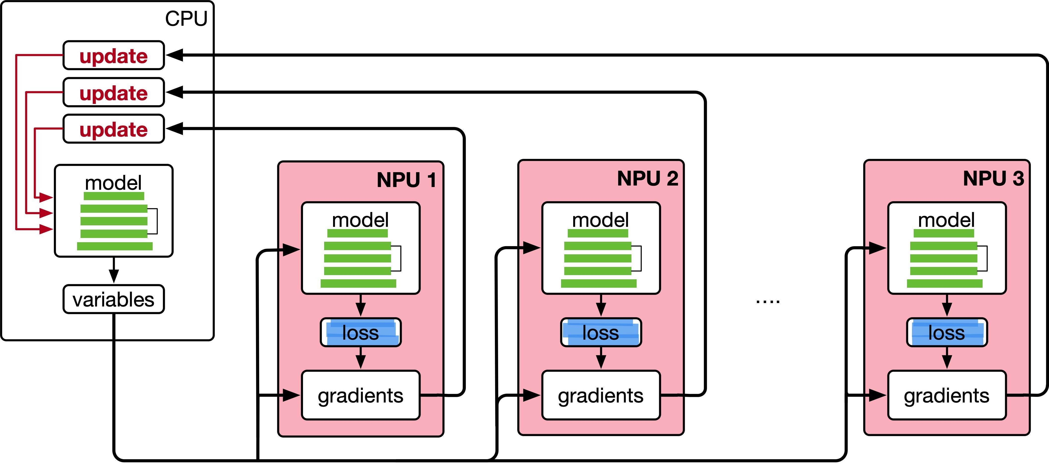
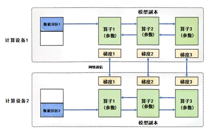
数据并行的核心思想是将整个神经网络模型复制到多个计算设备上,并将训练数据分成若干子集,分配到每个计算设备上。每个计算设备独立进行前向传播和反向传播,计算出本地的梯度,并将所有设备的梯度汇总以更新模型。这个过程的关键在于梯度的同步和平均。

在数据并行系统中,每个计算设备都有整个神经网络模型的模型副本(Model Replica),进行并行计算。每个计算设备只分配一个批次数据样本的子集,并根据该批次数据样本进行网络模型的前向计算。假设一个批次的训练样本数量为N,使用M个计算设备并行计算,每个计算设备会分配到 个样本。前向计算完成后,每个计算设备根据本地样本计算损失值,得到速度 (为加速卡编号),并将本地模型进行同步。所有计算设备需要合并其他速度卡给出的速度值,然后使用平均值对模型进行更新,完成该批次训练。图1给出了由两个计算设备生成的数据并行训练系统样例。

框架图

训练过程的数学公式

假设我们有一个神经网络模型 ,其中 是输入, 是模型的参数。数据并行的训练过程可以分为以下几个步骤:

前向传播

每个设备 计算其子集数据 的前向传播,得到输出

损失计算

每个设备 根据其本地数据计算损失

其中, 是目标标签, 是损失函数。

反向传播

每个设备根据本地数据计算梯度 ,并将这些梯度广播到所有设备。

梯度聚合

所有设备的梯度将被汇总(通常是通过平均),然后每个设备的梯度更新模型参数

其中, 是设备的总数。

模型更新

使用汇总后的平均梯度更新模型参数:

其中, 是学习率。

数据并行代码的对应

在 PyTorch 中,数据并行的实现通常使用 nn.DataParallelnn.DistributedDataParallel。通过这些工具,我们可以将上述的数学过程映射到实际的代码中。

前向传播和损失计算

1
2
3
4
5
6
7
8
9
class Model(nn.Module):
def init(self, input_size, output_size):
super(Model, self).init()
self.fc = nn.Linear(input_size, output_size) # 线性层

def forward(self, input):
output = self.fc(input)
return output

· 前向传播公式:每个设备计算 ,其中 是设备 上的数据。

使用 DataParallel 进行数据并行

1
2
3
if torch.cuda.device_count() > 1:
print("Let's use", torch.cuda.device_count(), "GPUs!")
model = nn.DataParallel(model) # 使用 DataParallel 进行数据并行

· 并行计算公式:模型被复制到每个设备上,并在每个设备上计算前向传播。

梯度计算和聚合

1
2
3
4
output = model(input) # 计算前向传播
loss = criterion(output, target) # 计算损失

loss.backward() # 计算梯度

反向传播公式:loss.backward() 计算每个设备上的梯度

梯度同步和平均

nn.DataParallel 中,PyTorch 会自动处理梯度的汇总。具体来说,它会在每次反向传播时将各设备上的梯度进行汇总,并同步到模型的主设备(通常是第一个设备)。

模型参数更新

1
optimizer.step() # 更新模型参数

· 参数更新公式:optimizer.step() 根据平均梯度来更新模型参数

结论

数据并行的核心思想是通过将数据划分为多个子集,并在多个计算设备上并行计算每个子集的前向传播和反向传播,最终聚合梯度并更新模型。在 PyTorch 中,nn.DataParallel 提供了自动化的方式来处理数据并行,包括前向传播的分配、梯度的聚合以及参数更新等。通过这个机制,我们可以高效地利用多个 GPU 来加速训练过程。

完整代码

1
2
3
4
5
6
7
8
9
10
11
12
13
14
15
16
17
18
19
20
21
22
23
24
25
26
27
28
29
30
31
32
33
34
35
36
37
38
39
40
41
42
43
44
45
46
47
48
49
50
51
52
53
54
55
56
57
58
59
60
61
62
63
64
65
66
67
68
69
70
71
import torch
import torch.nn as nn
import torch.optim as optim

# 定义模型类
class Model(nn.Module):
def __init__(self, input_size, output_size):
super(Model, self).__init__()
self.fc = nn.Linear(input_size, output_size) # 线性层

def forward(self, input):
output = self.fc(input)
# 在模型内打印输入和输出的尺寸
print("\tIn Model: input size", input.size(), "output size", output.size())
return output

# 初始化模型、损失函数和优化器
input_size = 10 # 输入大小示例
output_size = 2 # 输出大小示例
model = Model(input_size, output_size)

# 检查是否有多个GPU可用
if torch.cuda.device_count() > 1:
print("我们将使用", torch.cuda.device_count(), "个GPU!")
model = nn.DataParallel(model) # 使用DataParallel进行多GPU训练

# 如果有GPU可用,则将模型移至GPU
device = torch.device("cuda" if torch.cuda.is_available() else "cpu")
model.to(device)

# 定义损失函数和优化器
criterion = nn.MSELoss() # 均方误差损失
optimizer = optim.SGD(model.parameters(), lr=0.01) # 随机梯度下降优化器

# 示例输入和目标张量
input = torch.randn(64, input_size).to(device) # 批大小为64,输入大小为10
target = torch.randn(64, output_size).to(device) # 批大小为64,输出大小为2

# 前向传播
output = model(input) # 计算前向传播

# 计算损失
loss = criterion(output, target)

# 反向传播(计算梯度)
loss.backward()

# 更新模型参数
optimizer.step()

# 可选:打印损失和其他信息
print(f"总损失:{loss.item()}")

# 如果使用DataParallel,则显示每个设备上的损失
if torch.cuda.device_count() > 1:
# 检查每个GPU上的损失
losses = []
for i in range(torch.cuda.device_count()):
# 获取每个设备的输出和损失
loss_on_device = criterion(output.to(f'cuda:{i}'), target.to(f'cuda:{i}'))
losses.append(loss_on_device.item())
print(f"GPU-{i}上的损失:{loss_on_device.item()}")

# 计算所有GPU的聚合损失
total_loss_aggregated = sum(losses) / len(losses) # 或者直接使用sum(losses)来计算总损失
print(f"聚合后的损失:{total_loss_aggregated}")
else:
print(f"单个GPU/CPU上的损失:{loss.item()}")

# 打印batch的结果:输入尺寸和输出尺寸
print(f"Batch结果:输入尺寸 {input.size()},输出尺寸 {output.size()}")

当你运行这段代码时,你会看到类似以下的输出:

1
2
3
4
5
6
7
8
9
我们将使用 2 个GPU!
In Model: input size torch.Size([32, 10]) output size torch.Size([32, 2])
Outside: input size torch.Size([64, 10]) output_size torch.Size([64, 2])
总损失:1.234567
GPU-0上的损失:1.120987
GPU-1上的损失:1.345678
聚合后的损失:1.233333
Batch结果:输入尺寸 torch.Size([64, 10]),输出尺寸 torch.Size([64, 2])

数据并行训练实战

使用 DistributedSampler 和 DistributedDataParallel 进行分布式训练。通过 DistributedSampler,数据集会被均匀划分到每个GPU上,确保每个GPU处理不同的数据,从而实现数据并行;而 DistributedDataParallel 会在每个GPU上复制模型,并在训练过程中同步梯度,实现高效的分布式训练。

创建 DistributedSampler 类

DistributedSampler 旨在将数据集的样本分配到不同的计算设备上。它将数据集的样本随机打乱并按设备数量分配,确保每个设备得到不同的训练样本。以下是实现 DistributedSampler 类的代码:

1
2
3
4
5
6
7
8
9
10
11
12
13
14
15
16
17
18
19
20
21
22
23
24
25
26
27
28
29
30
31
32
33
34
35
36
37
38
39
40
41
42
43
44
45
46
47
48
49
50
51
52
53
import torch
import math
import torch.distributed as dist
from torch.utils.data import Sampler

class DistributedSampler(Sampler):
def __init__(self, dataset, num_replicas=None, rank=None, shuffle=True, seed=0):
if num_replicas is None:
if not dist.is_available():
raise RuntimeError("Requires distributed package to be available")
num_replicas = dist.get_world_size() # 获取进程数(等于GPU数量)

if rank is None:
if not dist.is_available():
raise RuntimeError("Requires distributed package to be available")
rank = dist.get_rank() # 获取当前进程的排名

self.dataset = dataset # 数据集
self.num_replicas = num_replicas # 进程数量(默认与world_size相同)
self.rank = rank # 当前进程编号
self.epoch = 0 # 当前训练轮次
self.num_samples = int(math.ceil(len(self.dataset) * 1.0 / self.num_replicas)) # 每个进程分配的样本数
self.total_size = self.num_samples * self.num_replicas # 数据集总大小
self.shuffle = shuffle # 是否打乱数据
self.seed = seed # 随机种子

def __iter__(self):
# 1. 打乱数据
if self.shuffle:
g = torch.Generator()
g.manual_seed(self.seed + self.epoch) # 根据轮次和种子打乱数据
indices = torch.randperm(len(self.dataset), generator=g).tolist()
else:
indices = list(range(len(self.dataset)))

# 数据补充,确保总样本数为num_samples * num_replicas
indices += indices[:(self.total_size - len(indices))]
assert len(indices) == self.total_size

# 根据rank分配数据
indices = indices[self.rank:self.total_size:self.num_replicas]
assert len(indices) == self.num_samples

return iter(indices)

def __len__(self):
return self.num_samples

def set_epoch(self, epoch):
"""
设置当前训练的epoch,确保每个训练轮次的打乱顺序不同。
"""
self.epoch = epoch

这个类实现了分布式数据加载器,通过__iter__方法根据进程的rank分配数据,确保每个进程处理的数据不重叠,并且每个进程处理的数据量相同。set_epoch方法用于设置当前训练的epoch,确保每个训练轮次的打乱顺序不同。

完整的训练程序样例 main.py

以下是利用 DistributedSampler 进行训练的完整示例:

1
2
3
4
5
6
7
8
9
10
11
12
13
14
15
16
17
18
19
20
21
22
23
24
25
26
27
28
29
30
31
32
33
34
35
36
37
38
39
40
41
42
43
44
45
46
47
48
49
50
51
52
53
54
55
56
57
58
59
60
61
62
63
64
65
66
67
68
69
70
71
72
73
74
75
76
77
78
79
80
81
82
83
84
85
86
87
88
89
90
91
92
93
94
95
96
97
98
99
100
101
102
import argparse
import os
import torch
import torch.nn as nn
import torch.optim
import torch.distributed as dist
import torch.utils.data
import torch.utils.data.distributed
from torch.utils.data.distributed import DistributedSampler
import torchvision
import torchvision.transforms as transforms
from torchvision import datasets, models

# 从环境变量中获取 local_rank
local_rank = int(os.environ["LOCAL_RANK"])

# 参数设置
parser = argparse.ArgumentParser(description='ResNet for CIFAR-10')
parser.add_argument('-j', '--workers', default=4, type=int, metavar='N', help='number of data loading workers (default: 4)')
parser.add_argument('--epochs', default=100, type=int, metavar='N', help='number of total epochs to run')
parser.add_argument('--start-epoch', default=0, type=int, metavar='N', help='manual epoch number (useful on restarts)')
parser.add_argument('-b', '--batch-size', default=64, type=int, metavar='N')

args = parser.parse_args()

# 初始化分布式训练
torch.distributed.init_process_group(backend="nccl") # 初始化进程组
print("Use GPU:{} for training".format(local_rank))

# 创建模型 (使用 ResNet18)
model = models.resnet18(pretrained=True) # 使用预训练的 ResNet18
model.fc = nn.Linear(model.fc.in_features, 10) # CIFAR-10 有 10 个类别

# 设置当前GPU
torch.cuda.set_device(local_rank)
model = model.cuda()

# 使用 DistributedDataParallel 进行分布式数据并行
model = nn.parallel.DistributedDataParallel(
model,
device_ids=[local_rank],
output_device=local_rank,
find_unused_parameters=True
)

# 损失函数和优化器
criterion = nn.CrossEntropyLoss().cuda()
optimizer = torch.optim.SGD(model.parameters(), lr=0.1, momentum=0.9, weight_decay=1e-4)

# 数据转换和加载
transform = transforms.Compose([
transforms.ToTensor(),
transforms.Normalize(mean=[0.485, 0.456, 0.406], std=[0.229, 0.224, 0.225])
])

# CIFAR-10 数据集
train_dataset = datasets.CIFAR10(root='./data', train=True, download=True, transform=transform)
train_sampler = DistributedSampler(train_dataset)

# 创建数据加载器
train_loader = torch.utils.data.DataLoader(
train_dataset,
batch_size=args.batch_size,
shuffle=False,
num_workers=args.workers,
pin_memory=True,
sampler=train_sampler
)

# 训练循环
for epoch in range(args.start_epoch, args.epochs):
# 设置训练的epoch
train_sampler.set_epoch(epoch)

# 训练模型
model.train()
for i, (inputs, targets) in enumerate(train_loader):
inputs = inputs.cuda(non_blocking=True)
targets = targets.cuda(non_blocking=True)

# 前向传播
outputs = model(inputs)

# 打印每个GPU的输入、输出和损失
if dist.get_rank() == 0: # 只在rank=0的进程中打印
print(f"GPU-{local_rank} - Epoch {epoch}, Batch {i}, Input size: {inputs.size()}, Output size: {outputs.size()}")

# 计算损失
loss = criterion(outputs, targets)

# 打印损失信息
if dist.get_rank() == 0: # 只在rank=0的进程中打印
print(f"GPU-{local_rank} - Epoch {epoch}, Batch {i}, Loss: {loss.item()}")

# 反向传播和优化
optimizer.zero_grad()
loss.backward()
optimizer.step()

# 每个epoch打印一次
if dist.get_rank() == 0: # 只在rank=0的进程中打印
print(f'Epoch {epoch}/{args.epochs}, Loss: {loss.item()}')

启动分布式训练

使用以下命令行启动训练程序:

1
torchrun --nproc_per_node=2 main.py

其中,--nproc_per_node=2表示使用2个进程进行训练,每个进程对应一个GPU。
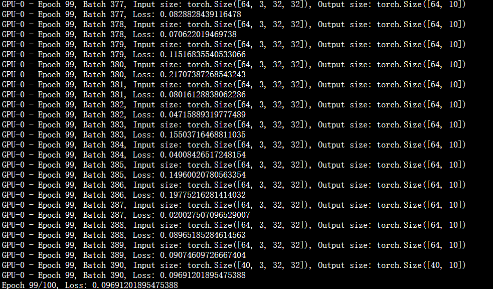
你会看到每个GPU的输入、输出和损失信息,以及每个epoch的损失信息。
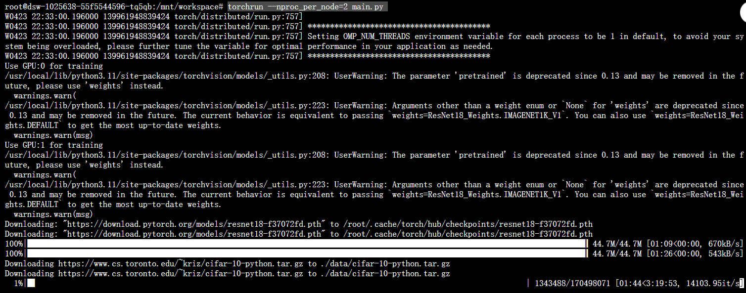
框架图
框架图

1
2
3
4
5
6
7
8
9
10
Use GPU:0 for training
GPU-0 - Epoch 0, Batch 0, Input size: torch.Size([3, 3, 224, 224]), Output size: torch.Size([3, 2, 224, 224])
GPU-0 - Epoch 0, Batch 0, Loss: 1.2321
GPU-0 - Epoch 0, Batch 1, Input size: torch.Size([3, 3, 224, 224]), Output size: torch.Size([3, 2, 224, 224])
GPU-0 - Epoch 0, Batch 1, Loss: 1.2137
GPU-1 - Epoch 0, Batch 0, Input size: torch.Size([3, 3, 224, 224]), Output size: torch.Size([3, 2, 224, 224])
GPU-1 - Epoch 0, Batch 0, Loss: 1.2345
GPU-1 - Epoch 0, Batch 1, Input size: torch.Size([3, 3, 224, 224]), Output size: torch.Size([3, 2, 224, 224])
GPU-1 - Epoch 0, Batch 1, Loss: 1.2154
Epoch 0/100, Loss: 1.2243

这里直接下载数据有点慢,可以手动下载数据集解压,然后修改代码中的数据集路径。
下载 CIFAR-10 数据集

1
wget https://www.cs.toronto.edu/~kriz/cifar-10-python.tar.gz

或者可以到这个链接下载:[cifar数据下载链接](https://www.cs.toronto.edu/~kriz/cifar-10-python.tar.gz)

解压 CIFAR-10 数据集

1
tar -xvzf cifar-10-python.tar.gz -C ./data

这个命令会将 CIFAR-10 数据集解压到 ./data 目录下。确认解压后的目录结构如下:

1
2
3
4
5
6
7
8
9
10
./data
├── cifar-10-batches-py
│ ├── batches.meta
│ ├── data_batch_1
│ ├── data_batch_2
│ ├── data_batch_3
│ ├── data_batch_4
│ ├── data_batch_5
│ └── test_batch
└── cifar-10-python.tar.gz

然后你就可以开始运行代码了。